scipy.signal.windows.

gaussian

scipy.signal.windows.gaussian(M, std, sym=True, *, xp=None, device=None)

Gibt ein Gaußsches Fenster zurück.

Parameter:

Mint

Anzahl der Punkte im Ausgabefenster. Wenn Null, wird ein leeres Array zurückgegeben. Bei negativen Werten wird eine Ausnahme ausgelöst.

stdfloat

Die Standardabweichung, sigma.

symbool, optional

Wenn True (Standard), wird ein symmetrisches Fenster zur Filterentwurf verwendet. Wenn False, wird ein periodisches Fenster für die Spektralanalyse generiert.

xparray_namespace, optional

Optionaler Array-Namespace. Sollte mit dem Array-API-Standard kompatibel sein oder von array-api-compat unterstützt werden. Standard: numpy

device: any

optionale Gerätespezifikation für die Ausgabe. Sollte mit einer der unterstützten Gerätespezifikationen in xp übereinstimmen.

Rückgabe:

wndarray

Das Fenster, dessen Maximalwert auf 1 normiert ist (obwohl der Wert 1 nicht erscheint, wenn M gerade und sym True ist).

Hinweise

Das Gaußsche Fenster ist definiert als

\[w(n) = e^{ -\frac{1}{2}\left(\frac{n}{\sigma}\right)^2 }\]

Beispiele

Probieren Sie es in Ihrem Browser aus!

Plotten Sie das Fenster und seine Frequenzantwort

>>> import numpy as np
>>> from scipy import signal
>>> from scipy.fft import fft, fftshift
>>> import matplotlib.pyplot as plt

>>> window = signal.windows.gaussian(51, std=7)
>>> plt.plot(window)
>>> plt.title(r"Gaussian window ($\sigma$=7)")
>>> plt.ylabel("Amplitude")
>>> plt.xlabel("Sample")

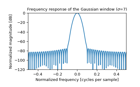
>>> plt.figure()
>>> A = fft(window, 2048) / (len(window)/2.0)
>>> freq = np.linspace(-0.5, 0.5, len(A))
>>> response = 20 * np.log10(np.abs(fftshift(A / abs(A).max())))
>>> plt.plot(freq, response)
>>> plt.axis([-0.5, 0.5, -120, 0])
>>> plt.title(r"Frequency response of the Gaussian window ($\sigma$=7)")
>>> plt.ylabel("Normalized magnitude [dB]")
>>> plt.xlabel("Normalized frequency [cycles per sample]")

ZurückIn Tab öffnen