scipy.signal.windows.

lanczos

scipy.signal.windows.lanczos(M, *, sym=True, xp=None, device=None)

Gibt ein Lanczos-Fenster zurück, das auch als Sinc-Fenster bekannt ist.

Parameter:

Mint

Anzahl der Punkte im Ausgabefenster. Wenn Null, wird ein leeres Array zurückgegeben. Bei negativen Werten wird eine Ausnahme ausgelöst.

symbool, optional

Wenn True (Standard), wird ein symmetrisches Fenster zur Filterentwurf verwendet. Wenn False, wird ein periodisches Fenster für die Spektralanalyse generiert.

xparray_namespace, optional

Optionaler Array-Namespace. Sollte mit dem Array-API-Standard kompatibel sein oder von array-api-compat unterstützt werden. Standard: numpy

device: any

optionale Gerätespezifikation für die Ausgabe. Sollte mit einer der unterstützten Gerätespezifikationen in xp übereinstimmen.

Rückgabe:

wndarray

Das Fenster, dessen Maximalwert auf 1 normiert ist (obwohl der Wert 1 nicht erscheint, wenn M gerade und sym True ist).

Hinweise

Das Lanczos-Fenster ist definiert als

\[w(n) = sinc \left( \frac{2n}{M - 1} - 1 \right)\]

wo

\[sinc(x) = \frac{\sin(\pi x)}{\pi x}\]

Das Lanczos-Fenster hat reduzierte Gibbs-Oszillationen und wird häufig zur Filterung von Klimazeitreihen mit guten Eigenschaften in der physikalischen und spektralen Domäne verwendet.

Hinzugefügt in Version 1.10.

Referenzen

[1]

Lanczos, C., und Teichmann, T. (1957). Applied analysis. Physics Today, 10, 44.

[2]

Duchon C. E. (1979) Lanczos Filtering in One and Two Dimensions. Journal of Applied Meteorology, Vol 18, pp 1016-1022.

[3]

Thomson, R. E. und Emery, W. J. (2014) Data Analysis Methods in Physical Oceanography (Dritte Auflage), Elsevier, pp 593-637.

[4]

Wikipedia, „Fensterfunktion“, http://en.wikipedia.org/wiki/Window_function

Beispiele

Probieren Sie es in Ihrem Browser aus!

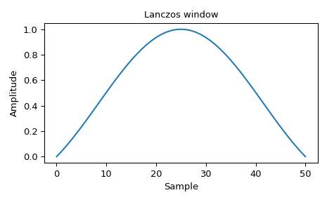
Zeichnet das Fenster

>>> import numpy as np
>>> from scipy.signal.windows import lanczos
>>> from scipy.fft import fft, fftshift
>>> import matplotlib.pyplot as plt
>>> fig, ax = plt.subplots(1)
>>> window = lanczos(51)
>>> ax.plot(window)
>>> ax.set_title("Lanczos window")
>>> ax.set_ylabel("Amplitude")
>>> ax.set_xlabel("Sample")
>>> fig.tight_layout()
>>> plt.show()

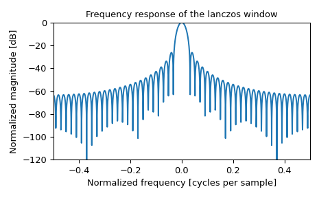
und seine Frequenzantwort

>>> fig, ax = plt.subplots(1)
>>> A = fft(window, 2048) / (len(window)/2.0)
>>> freq = np.linspace(-0.5, 0.5, len(A))
>>> response = 20 * np.log10(np.abs(fftshift(A / abs(A).max())))
>>> ax.plot(freq, response)
>>> ax.set_xlim(-0.5, 0.5)
>>> ax.set_ylim(-120, 0)
>>> ax.set_title("Frequency response of the lanczos window")
>>> ax.set_ylabel("Normalized magnitude [dB]")
>>> ax.set_xlabel("Normalized frequency [cycles per sample]")
>>> fig.tight_layout()
>>> plt.show()

ZurückIn Tab öffnen