scipy.special.voigt_profile#

scipy.special.voigt_profile(x, sigma, gamma, out=None) = <ufunc 'voigt_profile'>#

Voigt-Profil.

Das Voigt-Profil ist eine Faltung einer 1D-Normalverteilung mit Standardabweichung sigma und einer 1D-Cauchy-Verteilung mit halber Breite bei halber maximaler Höhe gamma.

Wenn sigma = 0, wird die Wahrscheinlichkeitsdichtefunktion (PDF) der Cauchy-Verteilung zurückgegeben. Umgekehrt, wenn gamma = 0, wird die PDF der Normalverteilung zurückgegeben. Wenn sigma = gamma = 0, ist der Rückgabewert Inf für x = 0 und 0 für alle anderen x.

Parameter:

xarray_like: Reeller Argument
sigmaarray_like: Die Standardabweichung des Normalverteilungsanteils
gammaarray_like: Die halbe Breite bei halber maximaler Höhe des Cauchy-Verteilungsanteils
outndarray, optional: Optionales Ausgabe-Array für die Funktionswerte

Rückgabe:

skalar oder ndarray: Das Voigt-Profil an den gegebenen Argumenten

Siehe auch

wofz: Faddeeva-Funktion

Hinweise

Es kann durch die Faddeeva-Funktion ausgedrückt werden

\[V(x; \sigma, \gamma) = \frac{Re[w(z)]}{\sigma\sqrt{2\pi}},\]

\[z = \frac{x + i\gamma}{\sqrt{2}\sigma}\]

wobei \(w(z)\) die Faddeeva-Funktion ist.

Referenzen

[1]

https://en.wikipedia.org/wiki/Voigt_profile

Beispiele

Berechnen Sie die Funktion am Punkt 2 für sigma=1 und gamma=1.

>>> from scipy.special import voigt_profile
>>> import numpy as np
>>> import matplotlib.pyplot as plt
>>> voigt_profile(2, 1., 1.)
0.09071519942627544

Berechnen Sie die Funktion an mehreren Punkten, indem Sie ein NumPy-Array für x angeben.

>>> values = np.array([-2., 0., 5])
>>> voigt_profile(values, 1., 1.)
array([0.0907152 , 0.20870928, 0.01388492])

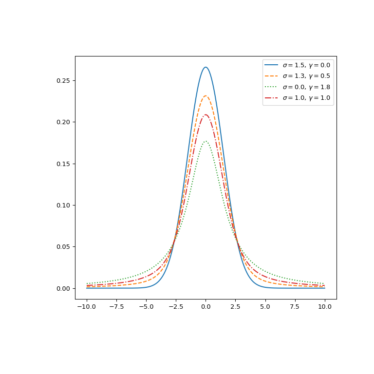
Zeichnen Sie die Funktion für verschiedene Parametersätze.

>>> fig, ax = plt.subplots(figsize=(8, 8))
>>> x = np.linspace(-10, 10, 500)
>>> parameters_list = [(1.5, 0., "solid"), (1.3, 0.5, "dashed"),
...                    (0., 1.8, "dotted"), (1., 1., "dashdot")]
>>> for params in parameters_list:
...     sigma, gamma, linestyle = params
...     voigt = voigt_profile(x, sigma, gamma)
...     ax.plot(x, voigt, label=rf"$\sigma={sigma},\, \gamma={gamma}$",
...             ls=linestyle)
>>> ax.legend()
>>> plt.show()

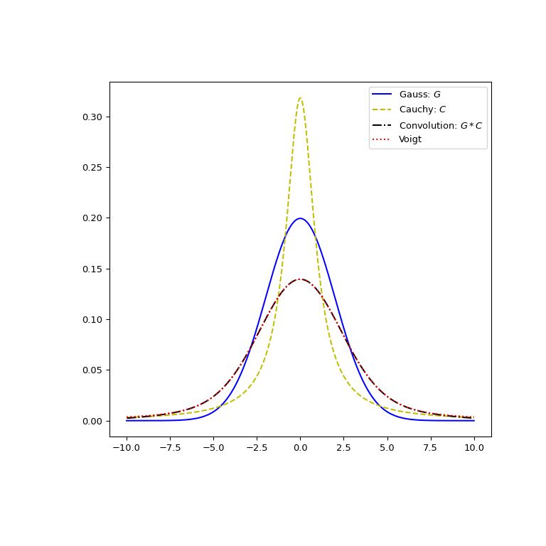
Überprüfen Sie visuell, dass das Voigt-Profil tatsächlich als Faltung einer Normal- und einer Cauchy-Verteilung entsteht.

>>> from scipy.signal import convolve
>>> x, dx = np.linspace(-10, 10, 500, retstep=True)
>>> def gaussian(x, sigma):
...     return np.exp(-0.5 * x**2/sigma**2)/(sigma * np.sqrt(2*np.pi))
>>> def cauchy(x, gamma):
...     return gamma/(np.pi * (np.square(x)+gamma**2))
>>> sigma = 2
>>> gamma = 1
>>> gauss_profile = gaussian(x, sigma)
>>> cauchy_profile = cauchy(x, gamma)
>>> convolved = dx * convolve(cauchy_profile, gauss_profile, mode="same")
>>> voigt = voigt_profile(x, sigma, gamma)
>>> fig, ax = plt.subplots(figsize=(8, 8))
>>> ax.plot(x, gauss_profile, label="Gauss: $G$", c='b')
>>> ax.plot(x, cauchy_profile, label="Cauchy: $C$", c='y', ls="dashed")
>>> xx = 0.5*(x[1:] + x[:-1])  # midpoints
>>> ax.plot(xx, convolved[1:], label="Convolution: $G * C$", ls='dashdot',
...         c='k')
>>> ax.plot(x, voigt, label="Voigt", ls='dotted', c='r')
>>> ax.legend()
>>> plt.show()