scipy.special.

diric#

scipy.special.diric(x, n)[Quelle]#

Periodische Sinc-Funktion, auch Dirichlet-Funktion genannt.

Die Dirichlet-Funktion ist definiert als

diric(x, n) = sin(x * n/2) / (n * sin(x / 2)),

wobei n eine positive ganze Zahl ist.

Parameter:

xarray_like: Eingabedaten
nint: Ganze Zahl, die die Periodizität definiert.

Rückgabe:

diricndarray

Beispiele

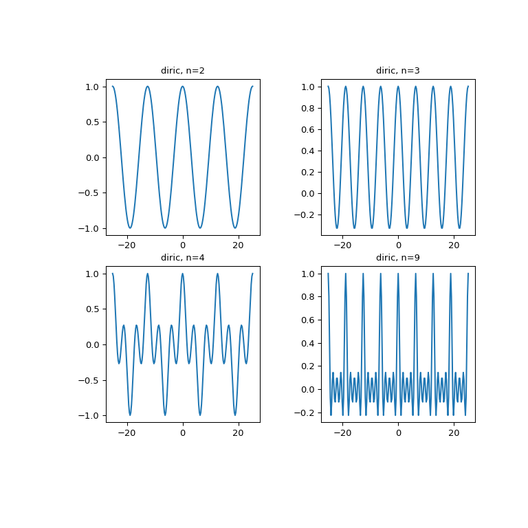
>>> import numpy as np
>>> from scipy import special
>>> import matplotlib.pyplot as plt

>>> x = np.linspace(-8*np.pi, 8*np.pi, num=201)
>>> plt.figure(figsize=(8, 8));
>>> for idx, n in enumerate([2, 3, 4, 9]):
...     plt.subplot(2, 2, idx+1)
...     plt.plot(x, special.diric(x, n))
...     plt.title('diric, n={}'.format(n))
>>> plt.show()

../../_images/scipy-special-diric-1_00_00.png

Das folgende Beispiel zeigt, dass diric die Amplituden (modulo Vorzeichen und Skalierung) der Fourier-Koeffizienten eines Rechteckimpulses liefert.

Unterdrücke die Ausgabe von Werten, die effektiv 0 sind

>>> np.set_printoptions(suppress=True)

Erstelle ein Signal x der Länge m mit k Einsen

>>> m = 8
>>> k = 3
>>> x = np.zeros(m)
>>> x[:k] = 1

Verwende die FFT, um die Fourier-Transformation von x zu berechnen, und inspiziere die Amplituden der Koeffizienten

>>> np.abs(np.fft.fft(x))
array([ 3.        ,  2.41421356,  1.        ,  0.41421356,  1.        ,
        0.41421356,  1.        ,  2.41421356])

Finde nun dieselben Werte (bis auf das Vorzeichen) mit diric. Wir multiplizieren mit k, um die unterschiedlichen Skalierungskonventionen von numpy.fft.fft und diric zu berücksichtigen.

>>> theta = np.linspace(0, 2*np.pi, m, endpoint=False)
>>> k * special.diric(theta, k)
array([ 3.        ,  2.41421356,  1.        , -0.41421356, -1.        ,
       -0.41421356,  1.        ,  2.41421356])