scipy.special.

laguerre#

scipy.special.laguerre(n, monic=False)[Quelle]#

Laguerre-Polynom.

Definiert als die Lösung von

\[x\frac{d^2}{dx^2}L_n + (1 - x)\frac{d}{dx}L_n + nL_n = 0;\]

\(L_n\) ist ein Polynom vom Grad \(n\).

Parameter:

nint: Grad des Polynoms.
monicbool, optional: Wenn True, wird der führende Koeffizient auf 1 skaliert. Standard ist False.

Rückgabe:

Lorthopoly1d: Laguerre-Polynom.

Siehe auch

genlaguerre: Verallgemeinertes (assoziiertes) Laguerre-Polynom.

Hinweise

Die Polynome \(L_n\) sind orthogonal über \([0, \infty)\) mit der Gewichtungsfunktion \(e^{-x}\).

Referenzen

[AS]

Milton Abramowitz und Irene A. Stegun, Hrsg. Handbook of Mathematical Functions with Formulas, Graphs, and Mathematical Tables. New York: Dover, 1972.

Beispiele

Die Laguerre-Polynome \(L_n\) sind der Spezialfall \(\alpha = 0\) der verallgemeinerten Laguerre-Polynome \(L_n^{(\alpha)}\). Wir überprüfen dies auf dem Intervall \([-1, 1]\)

>>> import numpy as np
>>> from scipy.special import genlaguerre
>>> from scipy.special import laguerre
>>> x = np.arange(-1.0, 1.0, 0.01)
>>> np.allclose(genlaguerre(3, 0)(x), laguerre(3)(x))
True

Die Polynome \(L_n\) erfüllen auch die Rekursionsrelation

\[(n + 1)L_{n+1}(x) = (2n +1 -x)L_n(x) - nL_{n-1}(x)\]

Dies kann für \(n = 3\) leicht auf \([0, 1]\) überprüft werden

>>> x = np.arange(0.0, 1.0, 0.01)
>>> np.allclose(4 * laguerre(4)(x),
...             (7 - x) * laguerre(3)(x) - 3 * laguerre(2)(x))
True

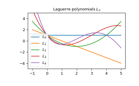
Dies ist die grafische Darstellung der ersten Laguerre-Polynome \(L_n\)

>>> import matplotlib.pyplot as plt
>>> x = np.arange(-1.0, 5.0, 0.01)
>>> fig, ax = plt.subplots()
>>> ax.set_ylim(-5.0, 5.0)
>>> ax.set_title(r'Laguerre polynomials $L_n$')
>>> for n in np.arange(0, 5):
...     ax.plot(x, laguerre(n)(x), label=rf'$L_{n}$')
>>> plt.legend(loc='best')
>>> plt.show()

../../_images/scipy-special-laguerre-1.png