jacobi#
- scipy.special.jacobi(n, alpha, beta, monic=False)[Quelle]#
Jacobi-Polynom.
Definiert als die Lösung von
\[(1 - x^2)\frac{d^2}{dx^2}P_n^{(\alpha, \beta)} + (\beta - \alpha - (\alpha + \beta + 2)x) \frac{d}{dx}P_n^{(\alpha, \beta)} + n(n + \alpha + \beta + 1)P_n^{(\alpha, \beta)} = 0\]für \(\alpha, \beta > -1\); \(P_n^{(\alpha, \beta)}\) ist ein Polynom vom Grad \(n\).
- Parameter:
- nint
Grad des Polynoms.
- alphafloat
Parameter, muss größer als -1 sein.
- betafloat
Parameter, muss größer als -1 sein.
- monicbool, optional
Wenn True, wird der führende Koeffizient auf 1 skaliert. Standard ist False.
- Rückgabe:
- Porthopoly1d
Jacobi-Polynom.
Hinweise
Für feste \(\alpha, \beta\) sind die Polynome \(P_n^{(\alpha, \beta)}\) über \([-1, 1]\) mit der Gewichtungsfunktion \((1 - x)^\alpha(1 + x)^\beta\) orthogonal.
Referenzen
[AS]Milton Abramowitz und Irene A. Stegun, Hrsg. Handbook of Mathematical Functions with Formulas, Graphs, and Mathematical Tables. New York: Dover, 1972.
Beispiele
Die Jacobi-Polynome erfüllen die Rekursionsrelation
\[P_n^{(\alpha, \beta-1)}(x) - P_n^{(\alpha-1, \beta)}(x) = P_{n-1}^{(\alpha, \beta)}(x)\]Dies kann zum Beispiel für \(\alpha = \beta = 2\) und \(n = 1\) über das Intervall \([-1, 1]\) verifiziert werden
>>> import numpy as np
>>> from scipy.special import jacobi
>>> x = np.arange(-1.0, 1.0, 0.01)
>>> np.allclose(jacobi(0, 2, 2)(x),
...             jacobi(1, 2, 1)(x) - jacobi(1, 1, 2)(x))
True
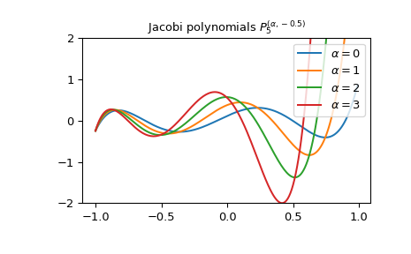
Plot des Jacobi-Polynoms \(P_5^{(\alpha, -0.5)}\) für verschiedene Werte von \(\alpha\)
>>> import matplotlib.pyplot as plt
>>> x = np.arange(-1.0, 1.0, 0.01)
>>> fig, ax = plt.subplots()
>>> ax.set_ylim(-2.0, 2.0)
>>> ax.set_title(r'Jacobi polynomials $P_5^{(\alpha, -0.5)}$')
>>> for alpha in np.arange(0, 4, 1):
...     ax.plot(x, jacobi(5, alpha, -0.5)(x), label=rf'$\alpha={alpha}$')
>>> plt.legend(loc='best')
>>> plt.show()