scipy.special.shichi#

scipy.special.shichi(x, out=None) = <ufunc 'shichi'>#

Hyperbolische Sinus- und Cosinus-Integrale.

Das hyperbolische Sinusintegral ist

\[\int_0^x \frac{\sinh{t}}{t}dt\]

und das hyperbolische Cosinusintegral ist

\[\gamma + \log(x) + \int_0^x \frac{\cosh{t} - 1}{t} dt\]

wobei \(\gamma\) die Euler-Mascheroni-Konstante ist und \(\log\) der Hauptzweig des Logarithmus ist [1].

Parameter:

xarray_like: Reelle oder komplexe Punkte, an denen die hyperbolischen Sinus- und Cosinusintegrale berechnet werden sollen.
outtuple von ndarray, optional: Optionale Ausgabe-Arrays für die Funktionsergebnisse

Rückgabe:

siSkalar oder ndarray: Hyperbolisches Sinusintegral bei x
ciSkalar oder ndarray: Hyperbolisches Cosinusintegral bei x

Siehe auch

sici: Sinus- und Cosinus-Integrale.
exp1: Exponentielle Integrale E1.
expi: Exponentielle Integrale Ei.

Hinweise

Für reelle Argumente mit x < 0 ist chi der Realteil des hyperbolischen Cosinusintegrals. Für solche Punkte unterscheiden sich chi(x) und chi(x + 0j) um den Faktor 1j*pi.

Für reelle Argumente wird die Funktion durch Aufruf der Cephes-Routine [2] shichi berechnet. Für komplexe Argumente basiert der Algorithmus auf den Mpmath-Routinen [3] shi und chi.

Referenzen

[1]

Milton Abramowitz und Irene A. Stegun, Hrsg. Handbook of Mathematical Functions with Formulas, Graphs, and Mathematical Tables. New York: Dover, 1972. (Siehe Abschnitt 5.2.)

[2]

Cephes Mathematical Functions Library, http://www.netlib.org/cephes/

[3]

Fredrik Johansson und andere. „mpmath: a Python library for arbitrary-precision floating-point arithmetic“ (Version 0.19) http://mpmath.org/

Beispiele

>>> import numpy as np
>>> import matplotlib.pyplot as plt
>>> from scipy.special import shichi, sici

shichi akzeptiert reelle oder komplexe Eingaben

>>> shichi(0.5)
(0.5069967498196671, -0.05277684495649357)
>>> shichi(0.5 + 2.5j)
((0.11772029666668238+1.831091777729851j),
 (0.29912435887648825+1.7395351121166562j))

Die hyperbolischen Sinus- und Cosinusintegrale Shi(z) und Chi(z) sind mit den Sinus- und Cosinusintegralen Si(z) und Ci(z) wie folgt verwandt:

Shi(z) = -i*Si(i*z)
Chi(z) = Ci(-i*z) + i*pi/2

>>> z = 0.25 + 5j
>>> shi, chi = shichi(z)
>>> shi, -1j*sici(1j*z)[0]            # Should be the same.
((-0.04834719325101729+1.5469354086921228j),
 (-0.04834719325101729+1.5469354086921228j))
>>> chi, sici(-1j*z)[1] + 1j*np.pi/2  # Should be the same.
((-0.19568708973868087+1.556276312103824j),
 (-0.19568708973868087+1.556276312103824j))

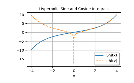
Funktionen, die auf der reellen Achse ausgewertet werden, plotten

>>> xp = np.geomspace(1e-8, 4.0, 250)
>>> x = np.concatenate((-xp[::-1], xp))
>>> shi, chi = shichi(x)

>>> fig, ax = plt.subplots()
>>> ax.plot(x, shi, label='Shi(x)')
>>> ax.plot(x, chi, '--', label='Chi(x)')
>>> ax.set_xlabel('x')
>>> ax.set_title('Hyperbolic Sine and Cosine Integrals')
>>> ax.legend(shadow=True, framealpha=1, loc='lower right')
>>> ax.grid(True)
>>> plt.show()

../../_images/scipy-special-shichi-1.png