scipy.special.sici#

scipy.special.sici(x, out=None) = <ufunc 'sici'>#

Sinus- und Cosinus-Integrale.

Das Sinusintegral ist

\[\int_0^x \frac{\sin{t}}{t}dt\]

und das Kosinusintegral ist

\[\gamma + \log(x) + \int_0^x \frac{\cos{t} - 1}{t}dt\]

wobei \(\gamma\) die Eulersche Konstante und \(\log\) der Hauptzweig des Logarithmus ist [1].

Parameter:

xarray_like: Reelle oder komplexe Punkte, an denen die Sinus- und Kosinusintegrale berechnet werden sollen.
outtuple von ndarray, optional: Optionale Ausgabe-Arrays für die Funktionsergebnisse

Rückgabe:

siSkalar oder ndarray: Sinusintegral bei x
ciSkalar oder ndarray: Kosinusintegral bei x

Siehe auch

shichi: Hyperbolische Sinus- und Cosinus-Integrale.
exp1: Exponentielle Integrale E1.
expi: Exponentielle Integrale Ei.

Hinweise

Für reelle Argumente mit x < 0 ist ci der Realteil des Kosinusintegrals. Für solche Punkte unterscheiden sich ci(x) und ci(x + 0j) um den Faktor 1j*pi.

Für reelle Argumente wird die Funktion durch Aufruf der Routine *sici* von Cephes [2] berechnet. Für komplexe Argumente basiert der Algorithmus auf den Routinen *si* und *ci* von Mpmath [3].

Referenzen

[1] (1,2)

Milton Abramowitz und Irene A. Stegun, Hrsg. Handbook of Mathematical Functions with Formulas, Graphs, and Mathematical Tables. New York: Dover, 1972. (Siehe Abschnitt 5.2.)

[2]

Cephes Mathematical Functions Library, http://www.netlib.org/cephes/

[3]

Fredrik Johansson und andere. „mpmath: a Python library for arbitrary-precision floating-point arithmetic“ (Version 0.19) http://mpmath.org/

Beispiele

>>> import numpy as np
>>> import matplotlib.pyplot as plt
>>> from scipy.special import sici, exp1

sici akzeptiert reelle oder komplexe Eingaben

>>> sici(2.5)
(1.7785201734438267, 0.2858711963653835)
>>> sici(2.5 + 3j)
((4.505735874563953+0.06863305018999577j),
(0.0793644206906966-2.935510262937543j))

Für z in der rechten Halbebene sind das Sinus- und Kosinusintegral mit dem Exponentialintegral E1 (in SciPy als scipy.special.exp1 implementiert) durch

Si(z) = (E1(i*z) - E1(-i*z))/2i + pi/2
Ci(z) = -(E1(i*z) + E1(-i*z))/2

verbunden. Siehe [1] (Gleichungen 5.2.21 und 5.2.23).

Wir können diese Beziehungen verifizieren

>>> z = 2 - 3j
>>> sici(z)
((4.54751388956229-1.3991965806460565j),
(1.408292501520851+2.9836177420296055j))

>>> (exp1(1j*z) - exp1(-1j*z))/2j + np.pi/2  # Same as sine integral
(4.54751388956229-1.3991965806460565j)

>>> -(exp1(1j*z) + exp1(-1j*z))/2            # Same as cosine integral
(1.408292501520851+2.9836177420296055j)

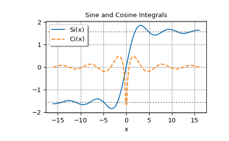
Plotten der auf der reellen Achse ausgewerteten Funktionen; die gestrichelten horizontalen Linien liegen bei pi/2 und -pi/2

>>> x = np.linspace(-16, 16, 150)
>>> si, ci = sici(x)

>>> fig, ax = plt.subplots()
>>> ax.plot(x, si, label='Si(x)')
>>> ax.plot(x, ci, '--', label='Ci(x)')
>>> ax.legend(shadow=True, framealpha=1, loc='upper left')
>>> ax.set_xlabel('x')
>>> ax.set_title('Sine and Cosine Integrals')
>>> ax.axhline(np.pi/2, linestyle=':', alpha=0.5, color='k')
>>> ax.axhline(-np.pi/2, linestyle=':', alpha=0.5, color='k')
>>> ax.grid(True)
>>> plt.show()