scipy.special.tklmbda#

scipy.special.tklmbda(x, lmbda, out=None) = <ufunc 'tklmbda'>#

Kumulative Verteilungsfunktion der Tukey-Lambda-Verteilung.

Parameter:

x, lmbdaarray_like: Parameter
outndarray, optional: Optionales Ausgabe-Array für die Funktionsergebnisse

Rückgabe:

cdfscalar oder ndarray: Wert der Tukey-Lambda-CDF

Siehe auch

scipy.stats.tukeylambda: Tukey-Lambda-Verteilung

Beispiele

>>> import numpy as np
>>> import matplotlib.pyplot as plt
>>> from scipy.special import tklmbda, expit

Berechnet die kumulative Verteilungsfunktion (CDF) der Tukey-Lambda-Verteilung an mehreren x-Werten für lmbda = -1,5.

>>> x = np.linspace(-2, 2, 9)
>>> x
array([-2. , -1.5, -1. , -0.5,  0. ,  0.5,  1. ,  1.5,  2. ])
>>> tklmbda(x, -1.5)
array([0.34688734, 0.3786554 , 0.41528805, 0.45629737, 0.5       ,
       0.54370263, 0.58471195, 0.6213446 , 0.65311266])

Wenn lmbda 0 ist, ist die Funktion die logistische Sigmoidfunktion, die in scipy.special als expit implementiert ist.

>>> tklmbda(x, 0)
array([0.11920292, 0.18242552, 0.26894142, 0.37754067, 0.5       ,
       0.62245933, 0.73105858, 0.81757448, 0.88079708])
>>> expit(x)
array([0.11920292, 0.18242552, 0.26894142, 0.37754067, 0.5       ,
       0.62245933, 0.73105858, 0.81757448, 0.88079708])

Wenn lmbda 1 ist, ist die Tukey-Lambda-Verteilung gleichmäßig auf dem Intervall [-1, 1], sodass die CDF linear ansteigt.

>>> t = np.linspace(-1, 1, 9)
>>> tklmbda(t, 1)
array([0.   , 0.125, 0.25 , 0.375, 0.5  , 0.625, 0.75 , 0.875, 1.   ])

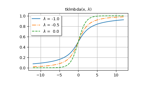
Im Folgenden generieren wir Grafiken für mehrere Werte von lmbda.

Die erste Abbildung zeigt Diagramme für lmbda <= 0.

>>> styles = ['-', '-.', '--', ':']
>>> fig, ax = plt.subplots()
>>> x = np.linspace(-12, 12, 500)
>>> for k, lmbda in enumerate([-1.0, -0.5, 0.0]):
...     y = tklmbda(x, lmbda)
...     ax.plot(x, y, styles[k], label=rf'$\lambda$ = {lmbda:-4.1f}')

>>> ax.set_title(r'tklmbda(x, $\lambda$)')
>>> ax.set_label('x')
>>> ax.legend(framealpha=1, shadow=True)
>>> ax.grid(True)

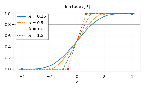
Die zweite Abbildung zeigt Diagramme für lmbda > 0. Die Punkte in den Diagrammen zeigen die Grenzen des Trägers der Verteilung.

>>> fig, ax = plt.subplots()
>>> x = np.linspace(-4.2, 4.2, 500)
>>> lmbdas = [0.25, 0.5, 1.0, 1.5]
>>> for k, lmbda in enumerate(lmbdas):
...     y = tklmbda(x, lmbda)
...     ax.plot(x, y, styles[k], label=fr'$\lambda$ = {lmbda}')

>>> ax.set_prop_cycle(None)
>>> for lmbda in lmbdas:
...     ax.plot([-1/lmbda, 1/lmbda], [0, 1], '.', ms=8)

>>> ax.set_title(r'tklmbda(x, $\lambda$)')
>>> ax.set_xlabel('x')
>>> ax.legend(framealpha=1, shadow=True)
>>> ax.grid(True)

>>> plt.tight_layout()
>>> plt.show()

../../_images/scipy-special-tklmbda-1_00_00.png

../../_images/scipy-special-tklmbda-1_00_01.png

Die CDF der Tukey-Lambda-Verteilung ist auch als cdf-Methode von scipy.stats.tukeylambda implementiert. Im Folgenden berechnen tukeylambda.cdf(x, -0.5) und tklmbda(x, -0.5) dieselben Werte

>>> from scipy.stats import tukeylambda
>>> x = np.linspace(-2, 2, 9)

>>> tukeylambda.cdf(x, -0.5)
array([0.21995157, 0.27093858, 0.33541677, 0.41328161, 0.5       ,
       0.58671839, 0.66458323, 0.72906142, 0.78004843])

>>> tklmbda(x, -0.5)
array([0.21995157, 0.27093858, 0.33541677, 0.41328161, 0.5       ,
       0.58671839, 0.66458323, 0.72906142, 0.78004843])

Die Implementierung in tukeylambda bietet auch Lage- und Skalenparameter sowie andere Methoden wie pdf() (die Wahrscheinlichkeitsdichtefunktion) und ppf() (die Umkehrfunktion der CDF). Für die Arbeit mit der Tukey-Lambda-Verteilung ist tukeylambda daher im Allgemeinen nützlicher. Der Hauptvorteil von tklmbda ist, dass es deutlich schneller ist als tukeylambda.cdf.