scipy.special.

y1p_zeros

scipy.special.y1p_zeros(nt, complex=False)

Berechnet `nt` Nullstellen der Bessel-Ableitung Y1’(z) und den Wert an jeder Nullstelle.

Die Werte sind gegeben durch Y1(z1) an jedem z1, wo Y1’(z1)=0.

Parameter:

ntint

Anzahl der zurückzugebenden Nullstellen

complexbool, Standardwert False

Setzen Sie auf False, um nur die reellen Nullstellen zurückzugeben; setzen Sie auf True, um nur die komplexen Nullstellen mit negativem Realteil und positivem Imaginärteil zurückzugeben. Beachten Sie, dass die komplexen Konjugierten der letzteren ebenfalls Nullstellen der Funktion sind, aber von dieser Routine nicht zurückgegeben werden.

Rückgabe:

z1pnndarray

Ort der nth Nullstelle von Y1’(z)

y1z1pnndarray

Wert der Ableitung Y1(z1) für die nth Nullstelle

Referenzen

[1]

Zhang, Shanjie und Jin, Jianming. „Computation of Special Functions“, John Wiley and Sons, 1996, Kapitel 5. https://people.sc.fsu.edu/~jburkardt/f77_src/special_functions/special_functions.html

Beispiele

Probieren Sie es in Ihrem Browser aus!

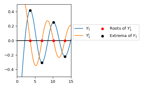
Berechnet die ersten vier Nullstellen von \(Y_1'\) und die Werte von \(Y_1\) an diesen Nullstellen.

>>> import numpy as np
>>> from scipy.special import y1p_zeros
>>> y1grad_roots, y1_values = y1p_zeros(4)
>>> with np.printoptions(precision=5):
...     print(f"Y1' Roots: {y1grad_roots.real}")
...     print(f"Y1 values: {y1_values.real}")
Y1' Roots: [ 3.68302  6.9415  10.1234  13.28576]
Y1 values: [ 0.41673 -0.30317  0.25091 -0.21897]

y1p_zeros kann verwendet werden, um die Extrempunkte von \(Y_1\) direkt zu berechnen. Hier plotten wir \(Y_1\) und die ersten vier Extrempunkte.

>>> import matplotlib.pyplot as plt
>>> from scipy.special import y1, yvp
>>> y1_roots, y1_values_at_roots = y1p_zeros(4)
>>> real_roots = y1_roots.real
>>> xmax = 15
>>> x = np.linspace(0, xmax, 500)
>>> x[0] += 1e-15
>>> fig, ax = plt.subplots()
>>> ax.plot(x, y1(x), label=r'$Y_1$')
>>> ax.plot(x, yvp(1, x, 1), label=r"$Y_1'$")
>>> ax.scatter(real_roots, np.zeros((4, )), s=30, c='r',
...            label=r"Roots of $Y_1'$", zorder=5)
>>> ax.scatter(real_roots, y1_values_at_roots.real, s=30, c='k',
...            label=r"Extrema of $Y_1$", zorder=5)
>>> ax.hlines(0, 0, xmax, color='k')
>>> ax.set_ylim(-0.5, 0.5)
>>> ax.set_xlim(0, xmax)
>>> ax.legend(ncol=2, bbox_to_anchor=(1., 0.75))
>>> plt.tight_layout()
>>> plt.show()

ZurückIn Tab öffnen