scipy.special.it2j0y0#

scipy.special.it2j0y0(x, out=None) = <ufunc 'it2j0y0'>#

Integrale im Zusammenhang mit Bessel-Funktionen erster Art der Ordnung 0.

Berechnet die Integrale

\[\begin{split}\int_0^x \frac{1 - J_0(t)}{t} dt \\ \int_x^\infty \frac{Y_0(t)}{t} dt.\end{split}\]

Mehr zu \(J_0\) und \(Y_0\) siehe j0 und y0.

Parameter:

xarray_like: Werte, an denen die Integrale ausgewertet werden sollen.
outTupel von ndarrays, optional: Optionale Ausgabearrays für die Funktionsergebnisse.

Rückgabe:

ij0Skalar oder ndarray: Das Integral für j0
iy0Skalar oder ndarray: Das Integral für y0

Referenzen

[1]

S. Zhang und J.M. Jin, „Computation of Special Functions“, Wiley 1996

Beispiele

Werten Sie die Funktionen an einem Punkt aus.

>>> from scipy.special import it2j0y0
>>> int_j, int_y = it2j0y0(1.)
>>> int_j, int_y
(0.12116524699506871, 0.39527290169929336)

Werten Sie die Funktionen an mehreren Punkten aus.

>>> import numpy as np
>>> points = np.array([0.5, 1.5, 3.])
>>> int_j, int_y = it2j0y0(points)
>>> int_j, int_y
(array([0.03100699, 0.26227724, 0.85614669]),
 array([ 0.26968854,  0.29769696, -0.02987272]))

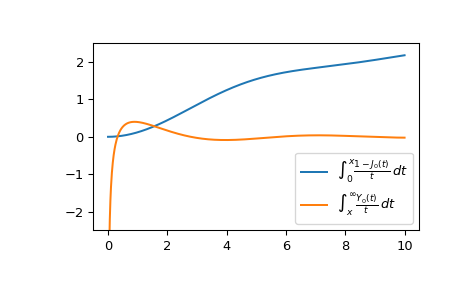
Plotten Sie die Funktionen von 0 bis 10.

>>> import matplotlib.pyplot as plt
>>> fig, ax = plt.subplots()
>>> x = np.linspace(0., 10., 1000)
>>> int_j, int_y = it2j0y0(x)
>>> ax.plot(x, int_j, label=r"$\int_0^x \frac{1-J_0(t)}{t}\,dt$")
>>> ax.plot(x, int_y, label=r"$\int_x^{\infty} \frac{Y_0(t)}{t}\,dt$")
>>> ax.legend()
>>> ax.set_ylim(-2.5, 2.5)
>>> plt.show()

../../_images/scipy-special-it2j0y0-1.png