scipy.special.itj0y0#

scipy.special.itj0y0(x, out=None) = <ufunc 'itj0y0'>#

Integrale von Bessel-Funktionen der ersten Art der Ordnung 0.

Berechnet die Integrale

\[\begin{split}\int_0^x J_0(t) dt \\ \int_0^x Y_0(t) dt.\end{split}\]

Weitere Informationen zu \(J_0\) und \(Y_0\) finden Sie unter j0 und y0.

Parameter:

xarray_like: Werte, an denen die Integrale ausgewertet werden sollen.
outTupel von ndarrays, optional: Optionale Ausgabearrays für die Funktionsergebnisse.

Rückgabe:

ij0Skalar oder ndarray: Das Integral von j0
iy0Skalar oder ndarray: Das Integral von y0

Referenzen

[1]

S. Zhang und J.M. Jin, „Computation of Special Functions“, Wiley 1996

Beispiele

Werten Sie die Funktionen an einem Punkt aus.

>>> from scipy.special import itj0y0
>>> int_j, int_y = itj0y0(1.)
>>> int_j, int_y
(0.9197304100897596, -0.637069376607422)

Werten Sie die Funktionen an mehreren Punkten aus.

>>> import numpy as np
>>> points = np.array([0., 1.5, 3.])
>>> int_j, int_y = itj0y0(points)
>>> int_j, int_y
(array([0.        , 1.24144951, 1.38756725]),
 array([ 0.        , -0.51175903,  0.19765826]))

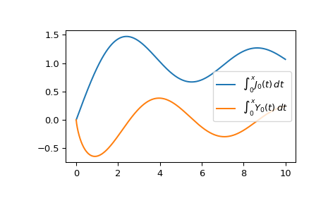
Plotten Sie die Funktionen von 0 bis 10.

>>> import matplotlib.pyplot as plt
>>> fig, ax = plt.subplots()
>>> x = np.linspace(0., 10., 1000)
>>> int_j, int_y = itj0y0(x)
>>> ax.plot(x, int_j, label=r"$\int_0^x J_0(t)\,dt$")
>>> ax.plot(x, int_y, label=r"$\int_0^x Y_0(t)\,dt$")
>>> ax.legend()
>>> plt.show()

../../_images/scipy-special-itj0y0-1.png