interp2d Übergangsleitfaden

Diese Seite enthält drei Sätze von Demonstrationen

• Low-Level FITPACK-Ersetzungen für scipy.interpolate.interp2d für eine fehlerkompatible Ersetzung von scipy.interpolate.interp2d aus Legacy-Code;

• empfohlene Ersetzungen für scipy.interpolate.interp2d für die Verwendung in neuem Code;

• eine Demonstration von Fehlerfällen bei FITPACK-basierter 2D-Linearintherpolation und empfohlenen Ersetzungen.

1. Wie man von der Verwendung von interp2d wegkommt

interp2d wechselt stillschweigend zwischen Interpolation auf einem regulären 2D-Gitter und Interpolation von 2D-gestreuten Daten. Der Wechsel basiert auf der Länge der (verflachten) Arrays x, y und z. Kurz gesagt, für reguläre Gitter verwenden Sie scipy.interpolate.RectBivariateSpline; für gestreute Interpolation verwenden Sie die bisprep/bisplev-Kombination. Im Folgenden geben wir Beispiele für den buchstäblichen Punkt-für-Punkt-Übergang, der die interp2d-Ergebnisse exakt beibehalten sollte.

1.1 interp2d auf einem regulären Gitter

Wir beginnen mit dem (leicht modifizierten) Docstring-Beispiel.

>>> import numpy as np
>>> import matplotlib.pyplot as plt
>>> from scipy.interpolate import interp2d, RectBivariateSpline

>>> x = np.arange(-5.01, 5.01, 0.25)
>>> y = np.arange(-5.01, 7.51, 0.25)
>>> xx, yy = np.meshgrid(x, y)
>>> z = np.sin(xx**2 + 2.*yy**2)
>>> f = interp2d(x, y, z, kind='cubic')

Dies ist der Code-Pfad für "reguläres Gitter", weil

>>> z.size == len(x) * len(y)
True

Beachten Sie auch, dass x.size != y.size

>>> x.size, y.size
(41, 51)

Lassen Sie uns nun eine Hilfsfunktion erstellen, um den Interpolator zu erstellen und ihn zu plotten.

>>> def plot(f, xnew, ynew):
...    fig, (ax1, ax2) = plt.subplots(1, 2, figsize=(8, 4))
...    znew = f(xnew, ynew)
...    ax1.plot(x, z[0, :], 'ro-', xnew, znew[0, :], 'b-')
...    im = ax2.imshow(znew)
...    plt.colorbar(im, ax=ax2)
...    plt.show()
...    return znew
...
>>> xnew = np.arange(-5.01, 5.01, 1e-2)
>>> ynew = np.arange(-5.01, 7.51, 1e-2)
>>> znew_i = plot(f, xnew, ynew)

Ersatz: Verwenden Sie RectBivariateSpline, das Ergebnis ist identisch

Beachten Sie die Transponierungen: erstens im Konstruktor, zweitens müssen Sie das Ergebnis der Auswertung transponieren. Dies dient dazu, die von interp2d durchgeführten Transponierungen rückgängig zu machen.

>>> r = RectBivariateSpline(x, y, z.T)
>>> rt = lambda xnew, ynew: r(xnew, ynew).T
>>> znew_r = plot(rt, xnew, ynew)

>>> from numpy.testing import assert_allclose
>>> assert_allclose(znew_i, znew_r, atol=1e-14)

Interpolationsreihenfolge: linear, kubisch usw.

interp2d verwendet standardmäßig kind="linear", was in beiden Richtungen, x- und y-, linear ist. RectBivariateSpline hingegen verwendet standardmäßig kubische Interpolation, kx=3, ky=3.

Hier ist die exakte Entsprechung

interp2d	RectBivariateSpline
keine kwargs	kx = 1, ky = 1
kind=’linear’	kx = 1, ky = 1
kind=’cubic’	kx = 3, ky = 3

1.2. interp2d mit vollständigen Koordinaten von Punkten (gestreute Interpolation)

Hier verflachen wir das Meshgrid aus der vorherigen Übung, um die Funktionalität zu veranschaulichen.

>>> xxr = xx.ravel()
>>> yyr = yy.ravel()
>>> zzr = z.ravel()
>>> f = interp2d(xxr, yyr, zzr, kind='cubic')

Beachten Sie, dass dies der Code-Pfad "kein reguläres Gitter" ist, der für gestreute Daten gedacht ist, mit len(x) == len(y) == len(z).

>>> len(xxr) == len(yyr) == len(zzr)
True

>>> xnew = np.arange(-5.01, 5.01, 1e-2)
>>> ynew = np.arange(-5.01, 7.51, 1e-2)
>>> znew_i = plot(f, xnew, ynew)

Ersatz: Verwenden Sie direkt scipy.interpolate.bisplrep / scipy.interpolate.bisplev

>>> from scipy.interpolate import bisplrep, bisplev
>>> tck = bisplrep(xxr, yyr, zzr, kx=3, ky=3, s=0)
# convenience: make up a callable from bisplev
>>> ff = lambda xnew, ynew: bisplev(xnew, ynew, tck).T   # Note the transpose, to mimic what interp2d does
>>> znew_b = plot(ff, xnew, ynew)

>>> assert_allclose(znew_i, znew_b, atol=1e-15)

Interpolationsreihenfolge: linear, kubisch usw.

interp2d verwendet standardmäßig kind="linear", was in beiden Richtungen, x- und y-, linear ist. bisplrep hingegen verwendet standardmäßig kubische Interpolation, kx=3, ky=3.

Hier ist die exakte Entsprechung

interp2d	bisplrep
keine kwargs	kx = 1, ky = 1
kind=’linear’	kx = 1, ky = 1
kind=’cubic’	kx = 3, ky = 3

2. Alternative zu interp2d: reguläres Gitter

Für neuen Code ist die empfohlene Alternative RegularGridInterpolator. Es handelt sich um eine unabhängige Implementierung, die nicht auf FITPACK basiert. Unterstützt Nachbar-, lineare Interpolation und Tensorprodukt-Splines ungerader Ordnung.

Die Spline-Knoten sind garantiert identisch mit den Datenpunkten.

Beachten Sie, dass hier

1. das Tupel-Argument ist (x, y)

2. das z-Array benötigt eine Transponierung

3. der Schlüsselname ist method, nicht kind

4. das Argument bounds_error ist standardmäßig auf True gesetzt.

>>> from scipy.interpolate import RegularGridInterpolator as RGI
>>> r = RGI((x, y), z.T, method='linear', bounds_error=False)

Auswertung: Erstellen Sie ein 2D-Meshgrid. Verwenden Sie indexing='ij' und sparse=True, um etwas Speicher zu sparen.

>>> xxnew, yynew = np.meshgrid(xnew, ynew, indexing='ij', sparse=True)

Auswerten, beachten Sie das Tupel-Argument

>>> znew_reggrid = r((xxnew, yynew))

>>> fig, (ax1, ax2) = plt.subplots(1, 2, figsize=(8, 4))
# Again, note the transpose to undo the `interp2d` convention
>>> znew_reggrid_t = znew_reggrid.T
>>> ax1.plot(x, z[0, :], 'ro-', xnew, znew_reggrid_t[0, :], 'b-')
>>> im = ax2.imshow(znew_reggrid_t)
>>> plt.colorbar(im, ax=ax2)

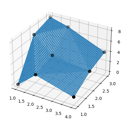
3. Gestreute 2D-Linearintherpolation: Bevorzugen Sie LinearNDInterpolator gegenüber SmoothBivariateSpline oder bisplrep

Für die gestreute 2D-Linearintherpolation können sowohl SmoothBivariateSpline als auch bisplrep entweder Warnungen ausgeben, die Daten nicht interpolieren oder Splines erzeugen, deren Knotenpunkte von den Datenpunkten abweichen. Bevorzugen Sie stattdessen LinearNDInterpolator, das auf der Triangulierung der Daten mittels QHull basiert.

# TestSmoothBivariateSpline::test_integral
>>> from scipy.interpolate import SmoothBivariateSpline, LinearNDInterpolator
>>> x = np.array([1,1,1,2,2,2,4,4,4])
>>> y = np.array([1,2,3,1,2,3,1,2,3])
>>> z = np.array([0,7,8,3,4,7,1,3,4])

Verwenden Sie nun die lineare Interpolation über eine QHull-basierte Triangulierung von Daten.

>>> xy = np.c_[x, y]   # or just list(zip(x, y))
>>> lut2 = LinearNDInterpolator(xy, z)
>>> X = np.linspace(min(x), max(x))
>>> Y = np.linspace(min(y), max(y))
>>> X, Y = np.meshgrid(X, Y)

Das Ergebnis ist leicht verständlich und interpretierbar.

>>> fig = plt.figure()
>>> ax = fig.add_subplot(projection='3d')
>>> ax.plot_wireframe(X, Y, lut2(X, Y))
>>> ax.scatter(x, y, z,  'o', color='k', s=48)

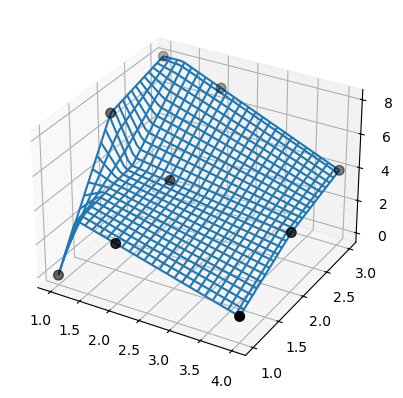
Beachten Sie, dass bisplrep etwas anderes tut! Es kann Spline-Knoten außerhalb der Daten platzieren.

Zur Veranschaulichung betrachten wir dieselben Daten aus dem vorherigen Beispiel.

>>> tck = bisplrep(x, y, z, kx=1, ky=1, s=0)
>>> fig = plt.figure()
>>> ax = fig.add_subplot(projection='3d')
>>> xx = np.linspace(min(x), max(x))
>>> yy = np.linspace(min(y), max(y))
>>> X, Y = np.meshgrid(xx, yy)
>>> Z = bisplev(xx, yy, tck)
>>> Z = Z.reshape(*X.shape).T
>>> ax.plot_wireframe(X, Y, Z, rstride=2, cstride=2)
>>> ax.scatter(x, y, z,  'o', color='k', s=48)

Außerdem gelingt es SmoothBivariateSpline nicht, die Daten zu interpolieren. Verwenden Sie erneut dieselben Daten aus dem vorherigen Beispiel.

>>> lut = SmoothBivariateSpline(x, y, z, kx=1, ky=1, s=0)
>>> fig = plt.figure()
>>> ax = fig.add_subplot(projection='3d')
>>> xx = np.linspace(min(x), max(x))
>>> yy = np.linspace(min(y), max(y))
>>> X, Y = np.meshgrid(xx, yy)
>>> ax.plot_wireframe(X, Y, lut(xx, yy).T, rstride=4, cstride=4)
>>> ax.scatter(x, y, z,  'o', color='k', s=48)

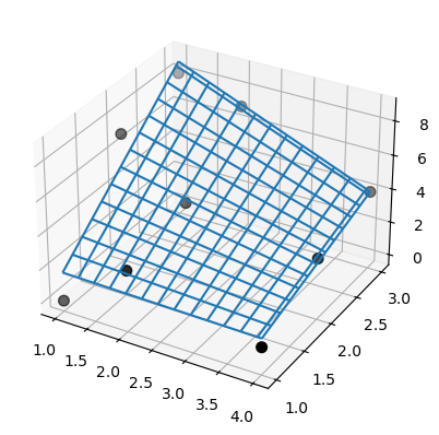
Beachten Sie, dass sowohl die Ergebnisse von SmoothBivariateSpline als auch von bisplrep Artefakte aufweisen, im Gegensatz zu LinearNDInterpolator. Die hier dargestellten Probleme wurden für die lineare Interpolation gezeigt, jedoch garantiert der FITPACK-Knotenauswahlmechanismus nicht, dass er diese Probleme für höherstufige (z. B. kubische) Spline-Oberflächen vermeidet.